ISS Eclipse Determination

Summary

The website projects.ansonbiggs.com discusses the importance of determining the eclipses a satellite will encounter during space missions, as this affects thermal and power budgets. An eclipse involves the umbra (complete darkness) and penumbra (partial shadow), with the International Space Station (ISS) spending minimal time in the penumbra due to its low orbit. The site explains the use of Two-Line Element (TLE) data to propagate the ISS's orbit and a function to calculate sunlight exposure. The ISS spends about 62% of its time in sunlight, with negligible time in the penumbra. The site also mentions that different orbits, such as polar or highly elliptical, can have varying sunlight exposure depending on the time of year.

Determining the eclipses a satellite will encounter is a major driving factor when designing a mission in space. Thermal and power budgets have to be made with the fact that a satellite will periodically be in the complete darkness of space where it will receive no solar radiation to power the solar panels and keep the spacecraft from freezing.

What is an Eclipse

{fig-alt=“A diagram of an eclipse. The sun is shown as a large yellow circle on the left. A smaller blue circle labeled”Body” is to the right of the sun. A spacecraft is shown above the body. The umbra and penumbra are labeled.”}

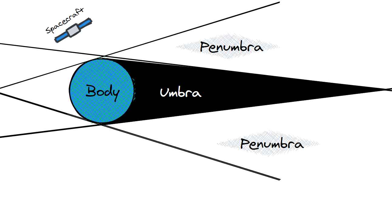
The above image is a simple representation of what an eclipse is. First, you’ll notice the Umbra is complete darkness, then the Penumbra, which is a shadow of varying darkness, and then the rest of the orbit is in full sunlight. For this example, I will be using the ISS, which has a very low orbit, so the Penumbra isn’t much of a problem. However, you can tell by looking at the diagram that higher altitude orbits would spend more time in the Penumbra.

Here is a more detailed view of the eclipse that will make it easier to explain what is going on. There are 2 Position vectors, and 2 radius that need to be known for simple eclipse determination. More advanced cases where the atmosphere of the body your orbiting can significantly affect the Umbra and Penumbra, and other bodies could also potentially block the Sun. However, we will keep it simple for this example since they have minimal effect on the ISS’s orbit. Rsun and Rbody are the radius of the Sun and Body (In this case Earth), respectively. r_sun_body is a vector from the center of the Sun to the center of the target body. For this example I will only be using one vector, but for more rigorous eclipse determination it is important to calculate the ephemeris at least once a day since it does significantly change over the course of a year. The reason that I am ignoring it at the moment is because there is currently no good way to calculate Ephemerides in Julia but the package is being worked on so I may revisit this and do a more rigorous analysis in the future. r_body_sc is a position vector from the center of the body being orbited, to the center of our spacecraft.

The Code

Imports

using Unitful
using LinearAlgebra
using SatelliteToolbox
using Plots
using Colors
theme(:ggplot2)

To get the orbit for the ISS, I used a Two-Line Element which is a data format for explaining orbits. The US Joint Space Operations Center makes these widely available, but https://live.ariss.org/tle/ makes the TLE for the ISS way more accessible (“ARISS TLE,” n.d.). The Julia Package SatelliteToolbox.jl makes it super easy to turn a TLE into an orbit that can be propagated. Simply putting the TLE in a string and using the tle string macro like below, we now have access to the information to start making our ISS orbit.

ISS = tle"""
ISS (ZARYA)
1 25544U 98067A   21103.84943184  .00000176  00000-0  11381-4 0  9990
2 25544  51.6434 300.9481 0002858 223.8443 263.8789 15.48881793278621
"""

TLE:
Name : ISS (ZARYA)
Satellite number : 25544
International designator : 98067A
Epoch (Year / Day) : 21 / 103.84943184 (2021-04-13T20:23:10.911)
Element set number : 999
Eccentricity : 0.00028580
Inclination : 51.64340000 deg
RAAN : 300.94810000 deg
Argument of perigee : 223.84430000 deg
Mean anomaly : 263.87890000 deg
Mean motion (n) : 15.48881793 revs / day
Revolution number : 27862
B* : 1.1381e-05 1 / er
ṅ / 2 : 1.76e-06 rev / day²
n̈ / 6 : 0 rev / day³

Now that we have the TLE, we can pass that into SatelliteToolbox’s orbit propagator. Before propagating the orbit, we need to have a range of time steps to pass into the propagator. The TLE gives the mean motion, n, which is the revolutions per day, so using that, we can calculate the amount of time required for one orbit, which is all that we’re worried about for this analysis. The propagator returns a tuple containing the Orbital elements, a position vector with units meters, and a velocity vector with units meters per second. For this analysis were only worried about the position vector.

ISS.mean_motion

15.48881793

orbit = Propagators.init(Val(:SGP4), ISS);
time = 0:0.1:((24/ISS.mean_motion).*60*60);
propagated = Propagators.propagate!.(orbit, time);
r = first.(propagated); # Get distance from propagator

We just need to use the radii and vectors discussed earlier to determine if the ISS is in the penumbra or umbra. This is a lot of trigonometry and vector math that I won’t bore anyone with. However, using the diagrams above and following the code in the sunlight function, you should follow what’s happening. For a rigorous discussion, check out (Vallado 1997).

function sunlight(Rbody, r_sun_body, r_body_sc)
    Rsun = 695_700u"km"

    hu = Rbody * norm(r_sun_body) / (Rsun - Rbody)

    θe = acos((r_sun_body ⋅ r_body_sc) / (norm(r_sun_body) * norm(r_body_sc)))

    θu = atan(Rbody / hu)
    du = hu * sin(θu) / sin(θe + θu)

    θp = π - atan(norm(r_sun_body) / (Rsun + Rbody))
    dp = Rbody * sin(θp) / cos(θe - θp)

    S = 1
    if (θe < π / 2) && (norm(r_body_sc) < du)
        S = 0
    end
    if (θe < π / 2) && ((du < norm(r_body_sc)) && (norm(r_body_sc) < dp))
        S = (norm(r_body_sc .|> u"km") - du) / (dp - du) |> ustrip
    end

    return S
end

sunlight (generic function with 1 method)

Then we can pass all the values we’ve gathered into the function we just made.

S = r .|> R -> sunlight(6371u"km", [0.5370, 1.2606, 0.5466] .* 1e8u"km", R .* u"m");

Plotting the Results

The sunlight function returns values from 0 to 1, 0 being complete darkness, 1 being complete sunlight, and anything between being the fraction of light being received. Again since the ISS has a very low orbit, the amount of time spent in the penumbra is almost insignificant.

Code

# Get fancy with the line color. 
light_range = range(colorant"black", stop=colorant"orange", length=101);
light_colors = [light_range[unique(round(Int, 1 + s * 100))][1] for s in S];

plot(
    LinRange(0, 24, length(S)),
    S .* 100,
    linewidth=5,
    legend=false,
    color=light_colors,
);

xlabel!("Time (hr)");
ylabel!("Sunlight (%)");
title!("ISS Sunlight Over a Day")

ISS Sunlight

Looking at the plot, the vertical transition from 0% to 100% makes it pretty clear that the time in the penumbra is limited. Still, almost counterintuitively, it also looks like the ISS gets more sunlight than it does darkness. So, using the raw sunlight data, we can calculate precisely how much time is spent in each region.

Time in Sun:

sun = length(S[S.==1]) / length(S) * 100

62.04757721886597

Time in Darkness:

umbra = length(S[S.==0]) / length(S) * 100

37.627951167918546

Time in Penumbra:

penumbra = 100 - umbra - sun

0.32447161321548634

This means that even with the ISS’s low orbit, it still gets sunlight ~62% of the time and spends almost no time in the penumbra. This would vary a few percent depending on the time of year, but in a circular orbit like the ISS, the amount of sunlight would remain pretty constant. There are other orbits like a polar orbit, lunar orbit, or highly elliptic earth orbits that can have their time in the sunlight vary widely by the time of year.

References

“ARISS TLE.” n.d. Amateur Radio on the International Space Station. https://live.ariss.org/tle/.Vallado, David A. 1997. Fundamentals of Astrodynamics and Applications, 2nd. Ed. Edited by Wiley Larson. Dordrecht: Microcosm, Inc.

Reuse

CC BY 4.0

This content was originally posted on my projects website here. The above summary was generated by the Kagi Summarizer.